Activate function
Learning Analysis
Optimization Techniques
Activate function
Learning Analysis
Optimization Techniques
LAB
Mnist 실습
1. 차이점
| 항목 |
신경망 구조 |
신경망❌구조 |
| 모델 구조 |
4개 Dense 계층(512→256→128→10), Dropout 3회 |
1개 Dense 계층(10) |
| 활성화 함수 |
relu(은닉층), softmax(출력층) |
softmax(출력층) |
| Dropout 사용 |
있음(0.3 비율, 3회) |
없음 |
| Optimizer |
Adam(learning_rate=0.0003) |
SGD(기본값) |
| Epoch 수 |
35 |
30 |
| Batch Size |
128 |
64 |
| 모델 복잡도 |
높음 |
매우 단순(로지스틱 회귀와 유사) |
2. 모델 구조 및 복잡도
신경망❌구조: 은닉층 없이 입력(784차원)에서 바로 10개 유닛의 softmax 출력층으로 연결된 매우 단순한 구조. 이는 다중 클래스 로지스틱 회귀와 동일.
신경망 구조: 3개의 은닉층(512, 256, 128 유닛)과 Dropout(0.3) 레이어를 포함해, 심층 신경망 구조. 출력층은 10개 유닛의 softmax.
신경망❌구조
md = Sequential()
md.add(Dense(10, activation = 'softmax', input_shape = (28*28,)))
신경망 구조
md = Sequential()
md.add(Dense(512, activation='relu', input_shape=(28*28,)))
md.add(Dropout(0.3))
md.add(Dense(256, activation='relu'))
md.add(Dropout(0.3))
md.add(Dense(128, activation='relu'))
md.add(Dropout(0.3))
md.add(Dense(10, activation='softmax'))
3. 정규화(Dropout) 적용 유무
op_mnist.py는 과적합 방지를 위해 Dropout 레이어를 3번 사용.
mnist.py는 Dropout 레이어 ❌
4. Optimizer 및 하이퍼파라미터 설정
신경망❌구조
md.compile(loss='sparse_categorical_crossentropy', optimizer = 'sgd', metrics=['acc'])
hist = md.fit(train_x2, train_y, epochs = 30, batch_size = 64, validation_split = 0.2)
신경망 구조
md.compile(loss='sparse_categorical_crossentropy', optimizer=Adam(learning_rate=0.0003), metrics=['acc'])
hist = md.fit(train_x2, train_y, epochs = 35, batch_size = 128, validation_split = 0.2)
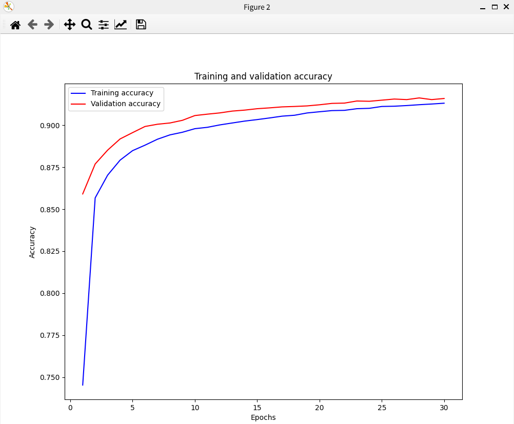
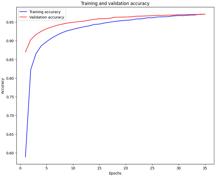
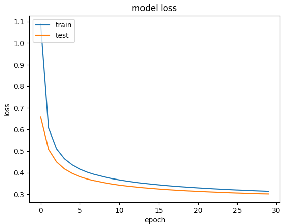
5. 결과 비교
| 신경망❌ 구조 |
신경망 구조 |
 |
 |
| 신경망❌ 구조 |
신경망 구조 |
 |
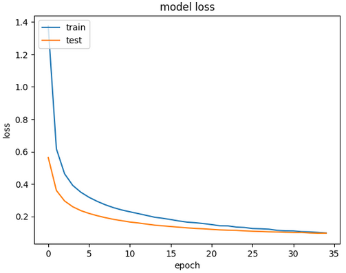 |
신경망❌ 구조

신경망 구조
6. 결론
- 신경망❌구조는 단일층 신경망(로지스틱 회귀) 구조로, 구현이 간단하고 빠르지만, 복잡한 데이터 표현력은 떨어진다.
- 신경망 구조는 심층 신경망(MLP) 구조에 Dropout과 Adam 옵티마이저를 적용해, 복잡한 패턴 학습과 과적합 방지에 중점을 둔 코드.
- 두 코드의 차이는 모델 구조(심층 vs. 단층), 정규화 적용, 옵티마이저 종류, 학습 파라미터 등에서 뚜렷하게 나타난다.
Cifar-10 실습
1. 차이점
| 항목 |
신경망 구조 |
신경망❌구조 |
| 모델 구조 |
4개 Dense 계층(512→256→128→10), Dropout 3회 |
1개 Dense 계층(10) |
| 활성화 함수 |
relu(은닉층), softmax(출력층) |
softmax(출력층) |
| Dropout 사용 |
있음(0.3 비율, 3회) |
없음 |
| Optimizer |
Adam(learning_rate=0.0003) |
SGD(기본값) |
| Epoch 수 |
35 |
30 |
| Batch Size |
128 |
64 |
| 모델 복잡도 |
높음 |
매우 단순(로지스틱 회귀와 유사) |
2. 모델 구조 및 복잡도
신경망❌구조: 은닉층 없이 입력(784차원)에서 바로 10개 유닛의 softmax 출력층으로 연결된 매우 단순한 구조. 이는 다중 클래스 로지스틱 회귀와 동일.
신경망 구조: 3개의 은닉층(512, 256, 128 유닛)과 Dropout(0.3) 레이어를 포함해, 심층 신경망 구조. 출력층은 10개 유닛의 softmax.
신경망❌구조
md = Sequential()
md.add(Dense(10, activation = 'softmax', input_shape = (32*32*3,)))
신경망 구조
md = Sequential()
md.add(Dense(512, activation='relu', input_shape=(3072,)))
md.add(Dropout(0.3))
md.add(Dense(256, activation='relu'))
md.add(Dropout(0.3))
md.add(Dense(128, activation='relu'))
md.add(Dropout(0.3))
md.add(Dense(10, activation='softmax'))
3. 정규화(Dropout) 적용 유무
신경망 구조(op_cifar_10.py): 과적합 방지를 위해 Dropout 레이어를 3번 사용.
신경망❌구조(cifar_10.py): Dropout 레이어가 없다.
4. Optimizer 및 하이퍼파라미터 설정
신경망❌구조
md.compile(loss='sparse_categorical_crossentropy', optimizer = 'sgd', metrics=['acc'])
hist = md.fit(train_x2, train_y, epochs = 30, batch_size = 64, validation_split = 0.2)
신경망 구조
md.compile(loss='sparse_categorical_crossentropy', optimizer=Adam(learning_rate=0.0003), metrics=['acc'])
hist = md.fit(train_x2, train_y, epochs = 35, batch_size = 128, validation_split = 0.2)
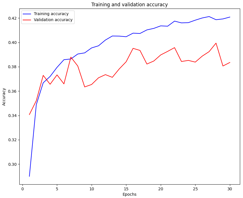
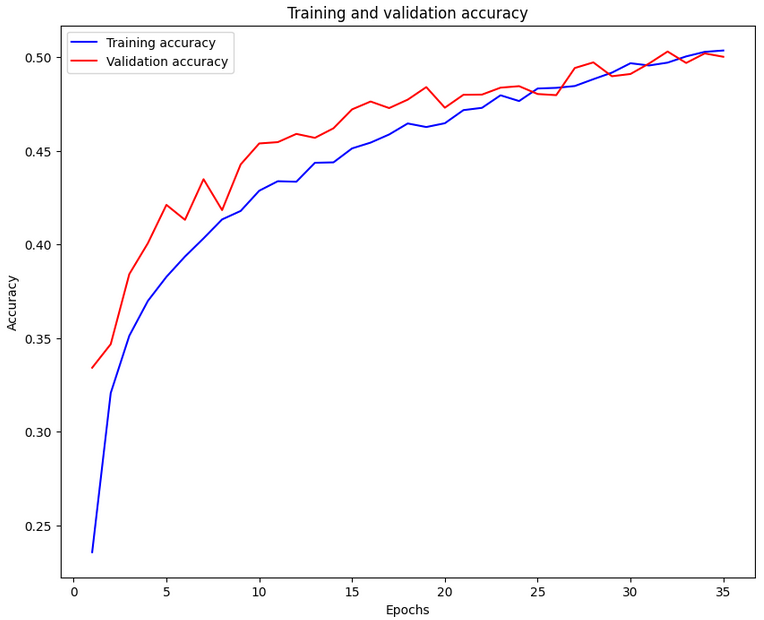
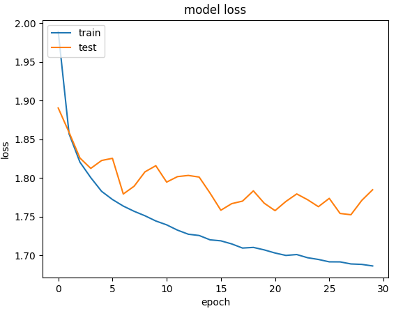
5. 결과 비교
| 신경망❌ 구조 |
신경망 구조 |
 |
 |
| 신경망❌ 구조 |
신경망 구조 |
 |
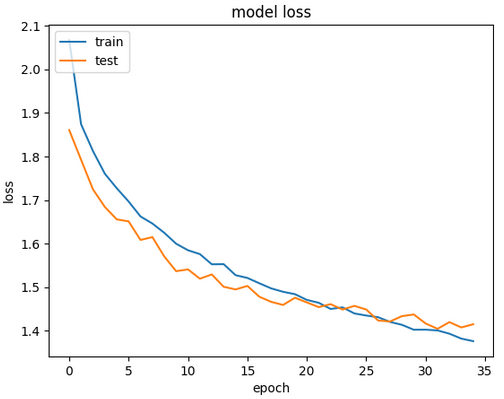 |
신경망❌ 구조

신경망 구조

6. 결론
신경망❌구조는 단일층 신경망(로지스틱 회귀) 구조로, 구현이 간단하고 빠르지만, 복잡한 데이터 표현력은 떨어진다.
신경망 구조는 심층 신경망(MLP) 구조에 Dropout과 Adam 옵티마이저를 적용해, 복잡한 패턴 학습과 과적합 방지.
두 코드의 차이는 모델 구조(심층 vs. 단층), 정규화 적용, 옵티마이저 종류, 학습 파라미터 등.